Prolate spheroids can be considered as simple geometries. On the other hand the flow around a prolate spheroid at incidence offers a complex three-dimensional turbulent shear flows, featuring stagnation flow, a highly three-dimensional boundary layer, cross-flow separation, the formation and evolution of free-vortex sheets and stream-wise vortices etc.

Since these flow features are important in the area of aerodynamic and hydrodynamic design of vehicles, they have been the basis of much research over the years and many experimental studies have provided comprehensive data that reveals the salient physics of these king of flows specially for 3:1 and 6:1 prolate spheroids. The 6:1 case has been most widely researched though.

I decided to play with OpenFOAM with a 6:1 case and compare the values with the test results. Some basic information can be seen in [Table.1] below. The chosen geometry is 2,40m long the Reynolds number is 4,2 millions.

Table.1) Some basic data related to the procedure. This page related to the 10° and 20° data. The 30° case has not been solved yet and may follow later.

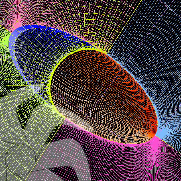
The 3D geometry and grid has been constructed with the open source tool Gmsh instead of blockMesh - snappyHexmesh. A half spherical domain has been used for the representation of the finite volumes. The mesh consists of 540.000 cells: 535.000 hex and 4.000 prisms.

Since only the high-Re turbulence models will be evaluated this time, near wall mesh has been constructed for an estimated average yPlus value for 30. Is this a good idea? Probably not because after the calculation for 10degrees of incidence, the real average yPlus value has been actualized as 17,55 which may impose problems for the turbulence models. But this was just a test anyway and the situation may also help for understanding the effect of such a low average yPlus value on the wall functions of turbulence models.

Figure.1) A view of 6:1 prolate spheroid and half spherical computational domain in Gmsh.

Three set of wind tunnel data by the angle of attack is available: 10°, 20° and 30°. Main interest will be the 20° case because this has the most complex flow features which may help to compare and separate different turbulence models and solution techniques more easily.

1. Angle of Attack 10 degrees

In the beginning eight high-Re turbulence models have been chosen to begin with the 10° case. These models are:

1. kEpsilon
2. kOmega
3. kOmegaSST
4. LienCubicKE
5. NonlinearKEShih
6. realizableKE
7. RNGkEpsilon
8. SpalartAllmaras

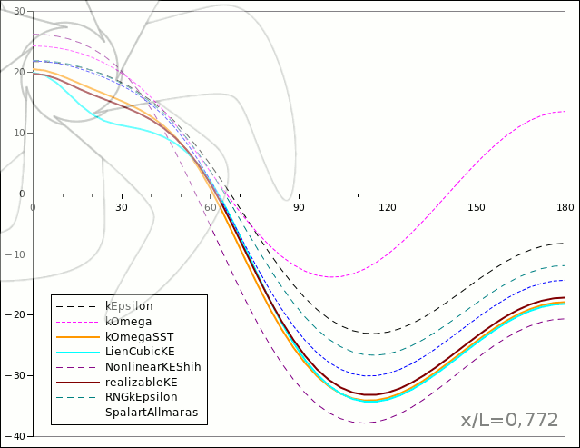
Figure.2) Circumferential pressure distribution on the section x/L=0,772 for 10degrees of incidence.

As can be seen on [Figure.2] obtained pressure results on the prolate spheroid are largely different for the same simulation setup by the turbulence models. Therefore four of the models have been eliminated for the next step.

2. Angle of Attack 20degrees

After the 10degrees case some turbulence models have been dropped and best three performer; kOmegaSST, LienCubicKE, realizableKE and also SpalartAllmaras has been chosen for the next cases. The grid has been modified for this case for getting a little higher yPlus value and after the simulations an average value of about 30 has been acquired. Grid size has not changed.

Next image shows the computed force coefficients. Indeed these coefficients are not the direct target of this study but it may provide a secondary benefit for understanding and comparing turbulence models, solvers and solution methods though. Calculated force coefficients are almost equal for the kOmegaSST and realizableKE, some different for the SpalartAllmaras and notably different with the LienCubicKE.

Figure.3) Calculated lift, drag and moment coefficients on the 6:1 prolate spheroid for AoA= 20degrees.

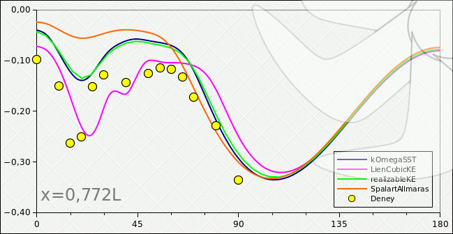
On the other hand the primary purpose of the study is testing the accuracy and limits of the used high-Re turbulence models with wall functions and relatively coarse grid. It must be noted that using wall functions may not be a good idea for such complex flow but one of the purpose of the study is trying to understand what can be achieved with an ordinary computer for such a complex flow conditions.

The results can be seen and understood on the figures below. For the presented conditions relatively best pressure distribution on the leeward side achieved by the Lien Cubic k epsilon model. The k omega SST and the Realizable k epsilon models shows very similar results and the standard implementation of Spalart Allmaras is the worst performer. It must be noted that fully-turbulent computations were performed which means that the turbulence model equations were active everywhere in the flow field. On the other hand the wind tunnel test data measured with forced transition by trip wire.

Figure.4) Circumferential pressure coefficient distribution on the section x/L=0,600 for 20degrees of incidence by turbulence models vs test results (yellow points)

Figure.5) Circumferential pressure coefficient distribution on the section x/L=0,772 for 20degrees of incidence by turbulence models vs test results (yellow points)

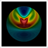
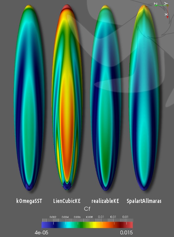
Figure.6) Calculated friction coefficient on the 6:1 prolate spheroid for AoA= 20degrees.

The first stage covered the steady state and the SIMPLE algorithm has been used here. For the 2.000 iterations the fastest model was SpalartAllmaras with 176min and the slowest was LienCubicKE with 234min. The processor was AMD Phenom II X6 1055T processor and only single core used.

At the next stages finer grids and low-Re turbulence models without wall functions and also unsteady solvers may be studied.

This page is a summary translation of the 10degrees and 20degrees cases originally written in Turkish.